
日常を数式を通して見るシリーズ。今回は円と楕円を行ったり来たりしながら、楕円の面積に関する性質を見ていく。シリーズの前回は 観覧車のゴンドラをぐわんぐわん揺らしたい - ヨーキョクデイ ということにしておく。
円と楕円と線型変換
まず、$a >0, b >0$ として、次の方程式で表される楕円を考える。
$$\frac{x^2}{a^2}+\frac{y^2}{b^2} = 1$$
この楕円は原点を中心とする単位円を x 軸方向に $a$ 倍、y 軸方向に $b$ 倍に拡大したものである。ここで、この単位円上の点 $(x_C, y_C)$ を考える。単位円を変形して楕円を作ったとき、この点が対応する楕円上の点を $(x_E, y_E)$ とする。すると、これらの点には次のような関係がある。
$$\begin{align}
\mqty(x_E \\ y_E)
&= \mqty(a x_C \\ b y_C) \\
&= \mqty(a & 0 \\ 0 & b) \mqty(x_C \\ y_C)
\end{align}$$
つまり、$A = \smqty(a & 0 \\ 0 & b)$ なる行列 $A$ で表される線型変換を考えていたことになる。
楕円の面積
それゆえ、この変換で写される図形の面積は元の面積の $\abs{\det A}$ 倍、つまり $ab$ 倍になる。実際に、単位円の面積は $\pi$ であるが、この楕円の面積は $\pi ab$ である。
中心角

$$\begin{align}
\mqty(x_E \\ y_E)
&= A \mqty(x_C \\ y_C) \\
&= \mqty(a \cos \theta_C \\ b \sin \theta_C)
\end{align}$$
一方で、楕円の中心と点 $(x_E, y_E)$ を結ぶ線分 $r_E$(半径のような何か、正式名称はわからない)が x 軸正の向きとのなす角を $\theta_E \in [0, 2\pi]$ とすると、$$
\begin{align}
\mqty(x_E \\ y_E )
&= \mqty(r_E \cos \theta_E \\ r_E \sin \theta_E) \\
&= r_E \mqty(\cos \theta_E \\ \sin \theta_E )
\end{align}$$となるから、$$\cos \theta_E : \sin \theta_E = a \cos \theta_C : b \sin \theta_C$$あるいは、これを変形して、$$\cos \theta_C : \sin \theta_C = b \cos \theta_E : a \sin \theta_E$$という関係が導かれる。分母が $0$ になりうるので $\tan$ で書かなかった。変換前後で点の象限は変化しないので、普通の逆正接 $\arctan$ を用いずに、$\mathrm{arctan2} (y, x) \in [0, 2\pi)$ を使うことにして、$\theta_C, \theta_E \in [0, 2\pi)$ について、$$\begin{align}
\theta_E(\theta_C) &= \mathrm{arctan2} (b \sin \theta_C, a \cos \theta_C) \\
\theta_C(\theta_E) &= \mathrm{arctan2} (a \sin \theta_E, b \cos \theta_E)
\end{align}$$とでき、また、自然に$\theta_E(\theta_C = 2\pi) = 2\pi$、$\theta_C(\theta_E = 2\pi) = 2\pi$ と対応づけることにする。これによって x 軸に対しての中心角についての相互関係を得る。
半径と極方程式
さて、単位円の半径は一定して $1$ であるが、先ほどの楕円の半径のような何か $r_E$ を考えると、この長さは楕円上の点の座標に依存する。$r_E=\sqrt{{x_E}^2 + {y_E}^2}$ であるが、$(x_E, y_E) = (a \cos \theta_C, b \sin \theta_C)$ であったから、$\theta_C$ を用いて $$r_E = \sqrt{ a^2 \cos^2 \theta_C + b^2 \sin^2 \theta_C}$$ と書ける。また、$(x_E, y_E) = (r_E \cos \theta_E, r_E \sin \theta_E)$ とも書けたから、これを当初の楕円の方程式に代入して変形することで、$\theta_E$ を用いた式が楽に得られる。
$$r_E = \frac{ab}{\sqrt{ b^2 \cos^2 \theta_E + a^2 \sin^2 \theta_E}}$$
これは $0 \leq \theta_E \leq 2 \pi$ において楕円を表す極方程式となっている。
また、任意の区間 $[\theta_{E\,begin}, \theta_{E\,end}] \subset [0, 2\pi]$ については x 軸に対しての中心角が $\theta_{E\,begin}$ から $\theta_{E\,end}$ であるところの楕円弧を表す。
極方程式と扇形の面積
一般の極座標による関数 $r(\theta)$ について、極方程式 $r = r(\theta), \theta \in [\theta_{begin}, \theta_{end}]$ で表される連続な曲線を考える。ここで、この曲線と、同じく極方程式で表される 2 直線 $\theta = \theta_{begin}$、$ \theta = \theta_{end}$ とで囲まれる領域 $S$ の面積は次の積分で与えられる。
$$\begin{align}
S(\theta_{begin}, \theta_{end})
&= \iint_S \dd{S} \\
&= \int_{\theta_{begin}}^{\theta_{end}} \int_{0}^{r(\theta)} r \dd{r} \dd{\theta} \\
&= \int_{\theta_{begin}}^{\theta_{end}} \frac{1}{2} r(\theta)^2 \dd{\theta}
\end{align}$$
ここで、次を考える。
$$S_E(\theta_E) = \int_{0}^{\theta_E} \frac{1}{2} r_E(\theta)^2 \dd{\theta}$$
前述の公式より、$S_E(\theta_E)$ なる関数は x 軸に対しての中心角 $\theta_E$ であるときの楕円の扇形の面積を表す。ところで、この積分を愚直に計算する必要はない。楕円が行列 $A$ によって単位円を変換したものであり、扇形に関してもそうであるため、対応する部分の単位円の扇形の面積がわかれば、これを $\abs{\det A} = ab$ 倍すれば、楕円の扇型の面積もわかるのだった。伏線回収。改めて、(x 軸に対しての)中心角 $\theta_C$ であるときの単位円の扇形の面積を $S_C(\theta_C)$ とすれば、$$S_C(\theta_C) = \frac{\theta_C}{2}$$である。さらに、 $\theta_E \in [0, 2\pi)$ に対応するものとして $\theta_C(\theta_E) = \mathrm{arctan2} (a \sin \theta_E, b \cos \theta_E)$ を考えていたから、$$
\begin{align}
S_E(\theta_E)
&= ab S_C( \mathrm{arctan2} (a \sin \theta_E, b \cos \theta_E) ) \\
&= \frac{ab}{2} \mathrm{arctan2} (a \sin \theta_E, b \cos \theta_E)
\end{align}$$
また、$\theta_E = 2\pi$ については $\theta_C = 2\pi$ が対応していたから、$$
\begin{align}
S_E(2\pi)
&= ab S_C(2\pi) \\
&= \pi ab
\end{align}$$となるがゆえ、当初に求めた楕円の面積が導出できた。
扇形の面積、再考

$$\begin{align}
S_E(\theta_{E\,begin}, \theta_{E\,end})
&= \int_{\theta_{E\,begin}}^{\theta_{E\,end}} \frac{1}{2} r_E(\theta)^2 \dd{\theta} \\
&= \int_{0}^{\theta_{E\,end}} \frac{1}{2} r_E(\theta)^2 \dd{\theta} - \int_{0}^{\theta_{E\,begin}} \frac{1}{2} r_E(\theta)^2 \dd{\theta} \\
&= S_E(\theta_{E\,end}) - S_E(\theta_{E\,begin})
\end{align}$$
まあ、積分表記はなくても明らかだが。
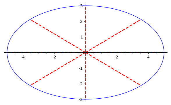
例題:楕円形のピザを等分割する
実はこれが本題だった。楕円形のピザを同じ面積のピースに切り分けたい事情があったときに役に立つ話だった。そんなピザがあるかは別として。とにかく、ピザの中心から放射状に切り分けるとして、これを $N (\geq 2)$ 個に分割するにはどういう角度で切っていけばいいのかというレシピを構成するための前置きが長くなったので、そのレシピというかアルゴリズムというかを書く。
- 楕円の長軸と短軸を割り出す
- そのどちらかを x 軸上に、もう一方を y 軸上に置き、中心を定める
- 長軸と短軸の長さから適当な $a$ と $b$ を算出する
- $N$ 回行われるのカットのうちのいずれか 1 つにおける、x 軸正の向きに対する角度 $\theta_{E\,0} \in [0, 2\pi)$ を適当に決める(この角度が基準となる)
- $\theta_{E\,0}$ より、$\theta_{C\,0} = \theta_{C}(\theta_{E\,0})$ を求める
- $k \in \{1, 2, \ldots, N-1\}$ なるすべての $k$ に対して $\theta_{C\,k} = \theta_{C\,0} + 2\pi k/N$ を求める
- $\theta_{C\,k} > 2\pi$ の場合は改めて $\theta_{C\,k} = \theta_{C\,k} - 2\pi$ とする
- それらの $\theta_{C\,k}$ について、$\theta_{E\,k} = \theta_{E}(\theta_{C\,k})$ を求める
- $\{\theta_{E\,0}, \theta_{E\,1}, \ldots, \theta_{E\,N-1}\}$ なる $N$ 個の角度こそが切るべき x 軸正の向きに対する角度である
下に $\frac{x^2}{5^2}+\frac{y^2}{3^2} = 1$ についての例を図示する。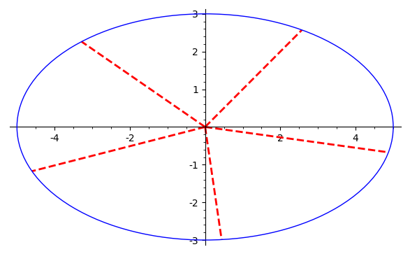
今回のための SageMath のコードを晒しておく。
def arctan2_nonneg(y, x):  # ∈ [0, 2*pi)
    t = arctan2(y, x)  # ∈ (-pi, pi]
    return t if t >= 0 else t + 2 * pi


assert arctan2_nonneg(0, 1) == 0
assert arctan2_nonneg(1, 0) == 1 / 2 * pi
assert arctan2_nonneg(0, -1) == pi
assert arctan2_nonneg(-1, -1) == 5 / 4 * pi

a = 5
b = 3


def _normalize(angle):  # ∈ [0, 2*pi]
    if angle < 0:
        return _normalize(angle + 2 * pi)
    elif 2 * pi < angle:
        return _normalize(angle - 2 * pi)
    else:
        return angle


def translate_central_angle_from_c_to_e(t):  # ∈ [0, 2*pi]
    t = _normalize(t)
    assert 0 <= t <= 2 * pi
    return 2 * pi if t == 2 * pi else arctan2_nonneg(b * sin(t), a * cos(t))


def translate_central_angle_from_e_to_c(t):  # ∈ [0, 2*pi]
    t = _normalize(t)
    assert 0 <= t <= 2 * pi
    return 2 * pi if t == 2 * pi else arctan2_nonneg(a * sin(t), b * cos(t))


# (x/a)**2 + (y/b)**2 = 1
def elliptical_sector(central_angle_rel_to_x_axis
                      ):  # central_angle_rel_to_x_axis ∈ [0, 2*pi]
    return a * b * unit_circular_sector(
        translate_central_angle_from_e_to_c(central_angle_rel_to_x_axis))


# x**2 + y**2 = 1
def unit_circular_sector(central_angle):  # central_angle ∈ [0, 2*pi]
    return _normalize(central_angle) / 2


n = 5
t_e_0 = pi / 4

t_c_0 = translate_central_angle_from_e_to_c(t_e_0)
t_e = [
    translate_central_angle_from_c_to_e(t_c_0 + k * 2 * pi / n)
    for k in range(n)
]
r_by_t_e = [a * b / sqrt((b * cos(t))**2 + (a * sin(t))**2) for t in t_e]
seg = [
    line([(0, 0), (r * cos(t), r * sin(t))],
         linestyle="--",
         rgbcolor=(1, 0, 0),
         thickness=2) for (r, t) in zip(r_by_t_e, t_e)
]

E = ellipse((0, 0), a, b)
G = E + reduce(lambda x, y: x + y, seg)
G.show(aspect_ratio=1)